Measures of Dispersion and its Types- Absolute and Relative

Dispersion is the act of dispersing from one location. One may say that people left the arrival place in dispersion. Similar to this, dispersion in statistics refers to the distribution of observations away from a central location.
The mean, median, and mode are three different metrics of central tendency, as we have seen in earlier blogs. However, not all values are equal to the central value; instead, most of them fall within its range, with some values being far from it. Furthermore, we employ a variety of dispersion techniques to determine the extent of the spread. The average's precision decreases with increasing spread.
A single number that represents the complete collection of data is used to calculate measures of central tendency. However, that primary value won't always match up with every observation. Some might differ more than others. Measures of dispersion are used to quantify this degree of variation. Assume that ten pupils in the class took the test, and the following scores were recorded: 45,55,50,65,75,54,39,99,12, 32. The class's average score, which was determined to be 52.6, was requested from the teacher. However, as you can see, not a single student has received this grade. Therefore, it might or might not be an appropriate data representation. And one needs to employ a suitable measure of dispersion in order to draw any conclusions about it. The better it is, the less variance there is.

Measures of dispersion are used to quantify how widely distributed or how much of a variance there is, or how widely distributed the numerical values are around a central value (the average).
The desirable properties of measure of dispersion are-
- · It must be precisely specified, using a set formula or computation technique. It shouldn't differ from person to person and should be the same for everyone who calculates it. If x and y (two people/systems) have the identical observations, then both x and y should use the same formula and obtain the same outcome.
- It should be based on all the data: The calculating method must take into account each of the 1500 observations if we are to determine the average for a group of 1500 people. It should be founded on each observation in order to be a representative sample of all the observations.
- · It should be least impacted by sampling fluctuations. A population is the total set of observations used as the basis for our study; that is, the entire set of observations. A sample is a subset of the population that demonstrates the characteristics of the population. A sample may only be considered good if it possesses every attribute of the population. A population is made up of numerous samples of different sizes, and each investigator may choose a different sample. Consequently, the measure ought to be least impacted by it and ought to provide almost identical results for various samples.
‘There are two main types of dispersion methods in
statistics which are:
- Absolute Measure of
Dispersion
- Relative Measure of Dispersion’
Absolute Measure of Dispersion: This method quantifies the variation using the same units of measurement as the observation. The dispersion's absolute measurements are:
·
Range
·
Quartile Deviation
·
Mean Deviation
·
Standard Deviation
·
Variance
§ Range: The range of a series is the difference between its highest and lowest observations..
Largest Value – Smallest Value

§
Quartile Deviation:
Partitioned values: The entire dataset is separated into an equal number of sections and sorted (either ascending or descending). A dataset is referred to as quartiles when it is divided into four equal parts, deciles when it is divided into ten equal parts, and percentiles when it is divided into one hundred equal parts.
When it comes to quartiles, 25% of the data fall under the first, 50% fall under the second, 75% fall under the third, and 100% fall under the fourth.
10% of the data falls under the first decile in deciles, 20% under the second, 30% under the third, 40% under the fourth, and so forth.
In terms of percentiles, 1% of the data falls under the first, 2% under the second, and so on.
Quartile
Deviation is half of the difference between the 3rd and 1st Quartile.

.png)
§
Mean deviation: The mean deviation is calculated by dividing the total number of observations by the sum of the absolute deviations of each observation from a central tendency measure.

.png)
It is minimum
when the deviations are measured from median.
a. Standard deviation: sum squared of the arithmetic mean deviation divided by the total number of observations.

b. Variance: The square of the standard deviation is the variance.

10.2.Relative Measure of Dispersion: Comparing the variation within and between distributions is the main use of relative measures of dispersion. They are commonly referred to as coefficients and are not specified in terms of any unit. The dispersion's relative measures are:
- · Coefficient of Range
- · Coefficient of Quartile Deviation
- · Coefficient of Mean Deviation
- · Coefficient of Standard Deviation
- · Coefficient of Variance
§
Coefficient of Range: Coefficient of
Range is the ratio of the difference between the highest and smallest
observations of the series to the sum of the highest and smallest observations
of the series.

a.
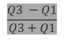
Coefficient of Quartile Deviation: Coefficient of
Quartile Deviation is the ratio of the difference between the 3rd and 1st
Quartile to the sum of the 3rd and 1st Quartile.
b.
Coefficient
of Mean Deviation:
Coefficient of Mean Deviation is the ratio of mean deviation to the
corresponding measure of central tendency.

Where M.D. stands for Mean Deviation.
c.
Coefficient
of Standard Deviation:
Coefficient of Standard deviation is the ratio of the standard deviation to the
corresponding mean of the data.
Where
SD stands for standard deviation, it is usually denoted by the symbol ![]() .
.
d.
Coefficient
of Variance: Coefficient of Variance is the ratio of the
Variance to the corresponding mean of the data.

Where
Var stands for Variance, it is usually denoted by the symbol ![]() .’
.’
10.3.Applications:
§
‘Range
gives us the length of an interval.
§ The interquartile range is a highly helpful tool for finding outliers. A data point that is extremely remote from every other point in a dataset is called an outlier. For instance, in a class, the majority of students had scores between 60 and 80, while one kid received a number between 0 and 100. This value would therefore have an impact on the average, rendering it an unreliable dataset representative. In this situation, we can compute the IQR, find these values, and utilize the IQR as a more accurate dataset representation.
The variance indicates the extent of the dataset's dispersion. A dataset with low variance indicates that the data are closely spaced and more representative of the average, whereas a dataset with high variance indicates that the data are more dispersed and distant from the average. Standard deviation computation is another usage for it. Since SD is the square root of variance, it is comparable to variance. When it comes to variance, we square the difference to make the measure's unit square, but when we take its root, the measure returns to its original unit. The better it is, the lower the value.
When analyzing ungrouped data, MD about mode would suffice,
while MD about median can be a useful tool for identifying outliers similar to
those in the IQR. The minimum MD is roughly the median. Let's say your friend
told you he wakes up at five every morning. However, you learned from a
different friend that he truly wakes up around 5:05 or 5:10 in the morning. You
didn't dispute the friend's information because there wasn't much of a
difference, but later on, his mother revealed that he doesn't really wake up
before nine. Would you still accept his information as accurate now? Obviously
not. Here, common sense is applied; nevertheless, in complex situations,
confidence intervals and standard deviation are used for assessment.
§ Coefficient of variation is used to compare consistency.
Suppose employee data has been collected from a group
of employees and an analysis was carried out. The variables included were age,
salary, number of promotions, number of awards received, department, manager
name, post.
Q1. What is average age of people working as ‘post x’?
Q2. Are there any outliers?
Q3. What is the average salary earned by people
working as ‘post y’?
Q4. Name the employee(‘s) with highest number of
awards?
Q7. Name the manager under whom employees have highest
number of awards in total?
Q8. Are all the people working under manager z as post
y earning similar salary amount?
Q9. Are there any biasness under manager z?
(Choose the appropriate statistical tools)
Let us consider the following example and calculate
the measures of Dispersion.
|
Class-limits
(C.L) |
mid-value
(x) |
Frequency(f) |
|
0-10 |
5 |
11 |
|
10-20 |
15 |
12 |
|
20-30 |
25 |
10 |
|
30-40 |
35 |
5 |
|
40-50 |
45 |
6 |
Quartile Deviation (QD) and Coefficient of QD:
|
Class-limits (C.L) |
mid-value (x) |
Frequency(f) |
Cumulative
frequency
|
|
0-10 |
5 |
11 |
11 |
|
10-20 |
15 |
12 |
23 |
|
20-30 |
25 |
10 |
33 |
|
30-40 |
35 |
5 |
38 |
|
40-50 |
45 |
6 |
44 |

Mean Deviation(MD) and Coefficient of MD:

|
Class-limits
(C.L) |
mid-value
(x) |
Frequency(f) |
f(|x-mean|)
|
|
0-10 |
5 |
11 |
557.5 |
|
10-20 |
15 |
12 |
2160 |
|
20-30 |
25 |
10 |
2500 |
|
30-40 |
35 |
5 |
875 |
|
40-50 |
45 |
6 |
1620 |
Mean Deviation (MD) = 175.28
Coefficient of Mean Deviation= 8.29
Standard Deviation (SD) and Coefficient of Variance:

|
Class-limits
(C.L) |
mid-value
(x) |
Frequency(f) |
Fx |
x-mean
|
|
0-10 |
5 |
11 |
55 |
33.86 |
|
10-20 |
15 |
12 |
180 |
158.86 |
|
20-30 |
25 |
10 |
250 |
228.86 |
|
30-40 |
35 |
5 |
175 |
153.86 |
|
40-50 |
45 |
6 |
270 |
248.86 |
Standard Deviation (SD) = 13.35
Coefficient of Variance = 8.43


Suppose your friend claimed that he always wakes up at 5am. But you got to know from another friend that he actually wakes up at 5.05 am or 5.10 am. Since, there is not much difference you didn't claim the information from the friend as false but later his mother said he actually does not wake up before 9. Now would you still claim his information as truth , of course not. Here we use our common sense but with complex situation we use measures of Dispersion.

.jpeg)

Comments
Post a Comment
If you have any doubt or suggestion kindly let me know. Happy learning!